Project Overview

The goal of this assignment is to get your hands dirty in different aspects of image warping with a “cool” application -- image mosaicing. You will take two or more photographs and create an image mosaic by registering, projective warping, resampling, and compositing them. Along the way, you will learn how to compute homographies, and how to use them to warp images.

Recover Homographies

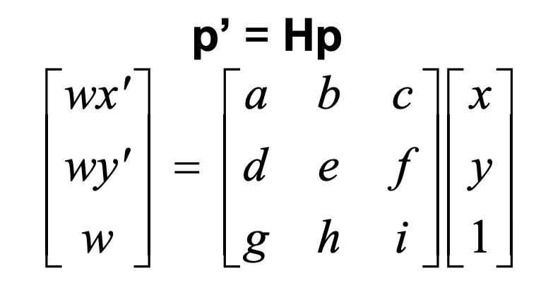
The above image is from lecture 11: Homographies and Panoramas, oct 9 2024

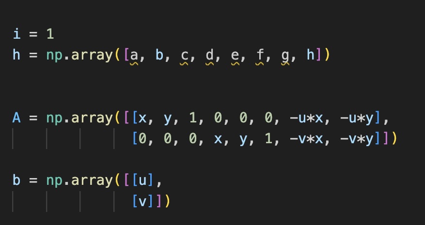
To solve for H the trick is to substitute the third coordinate in homogeneous coordinates z with x and y. If we substitute it into the x’ y’ coordinate and arrange the matrix this allows us to re express it as the least squares problem. Note that we can set scale factor i=1.

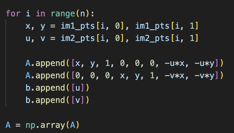
Note that we need at least 4 points (8 data points for 8 unknowns) for this to be determined or over determined. The left matrix and the right vector are extended by 2 rows for each additional correspondence:

Part 2. Image rectification

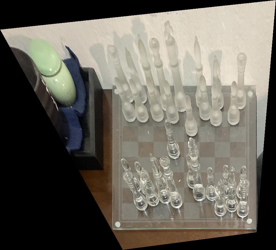
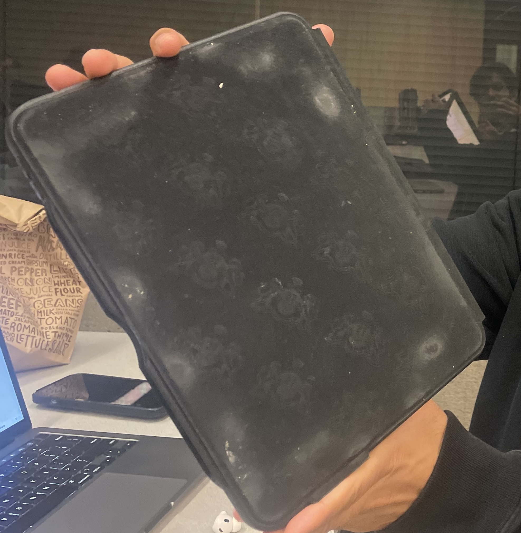
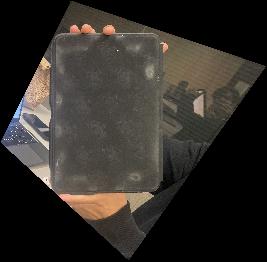
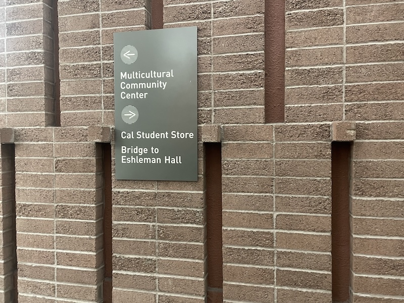
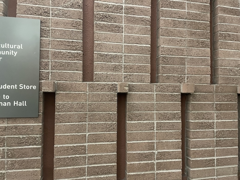
To rectify an image we take the point correspondences (for warping) between a flat planar surface of the image and a hand chosen rectangular region. Note that for warping I just reused my code from the previous project (inverse H + nearest neighbor interpolation for speed, I also tried linear but it’s to slow)

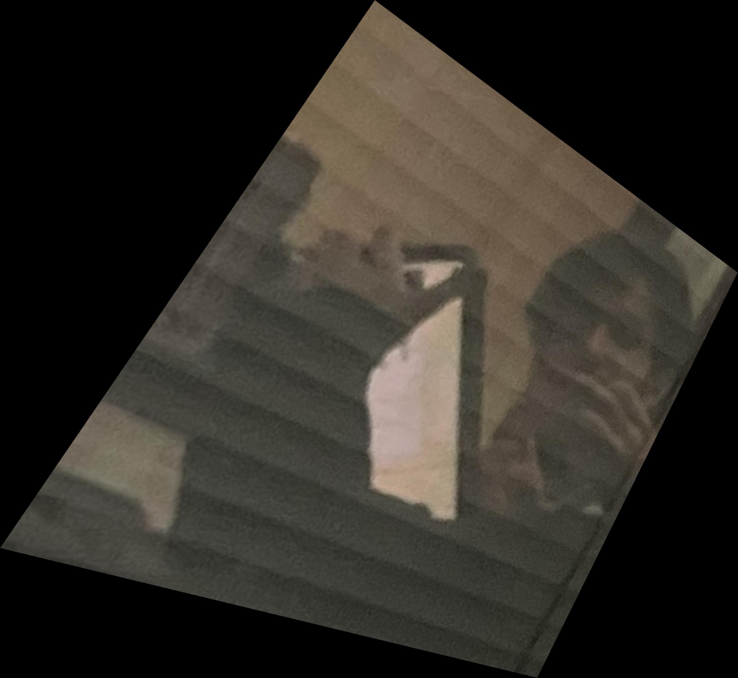
An especially annoying part of this process is that small mismatches/errors in the point correspondences lead to ridiculous projections. Both swapping out bad points, slowly moving the points into the desired projection worked really well to mitigate this (guided by visual debugging).

Mosaics

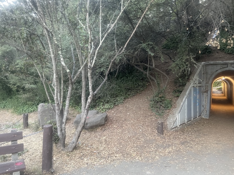
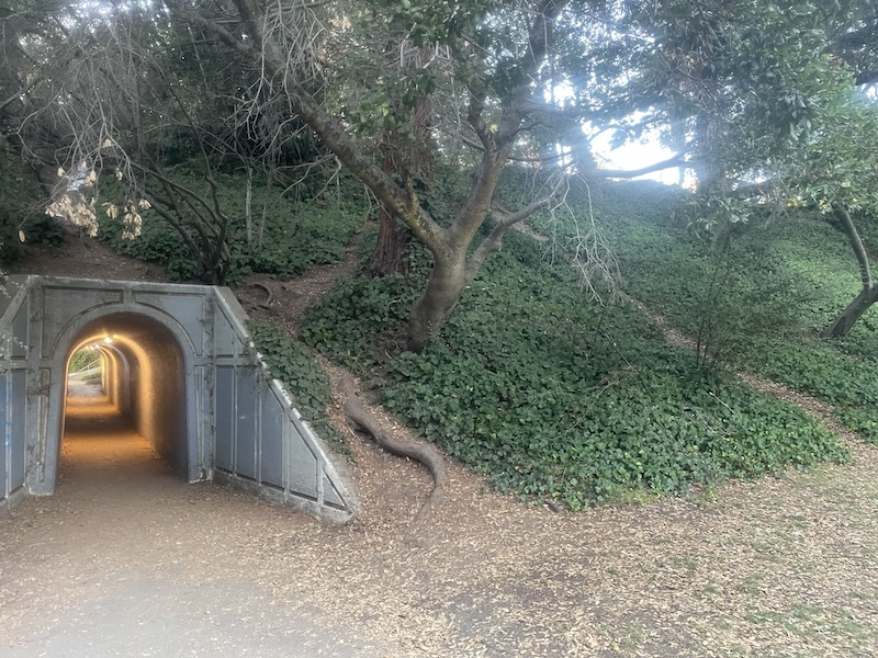
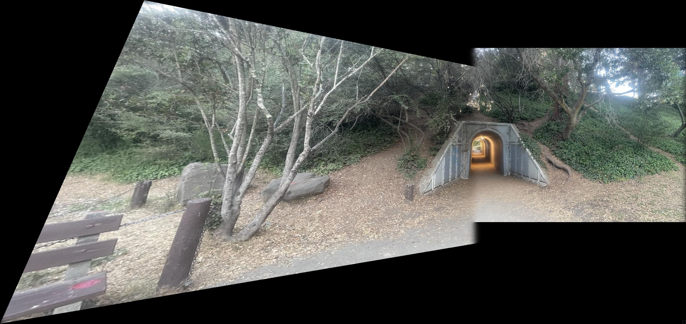
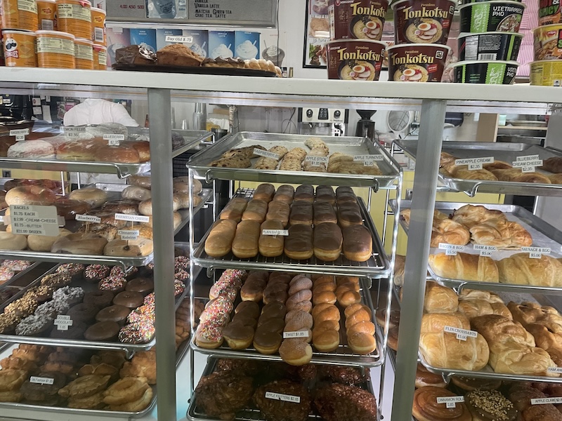
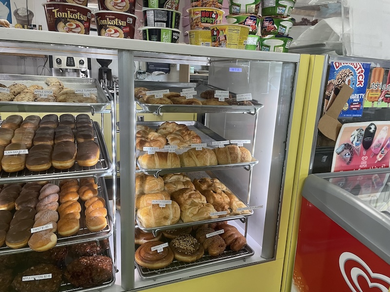
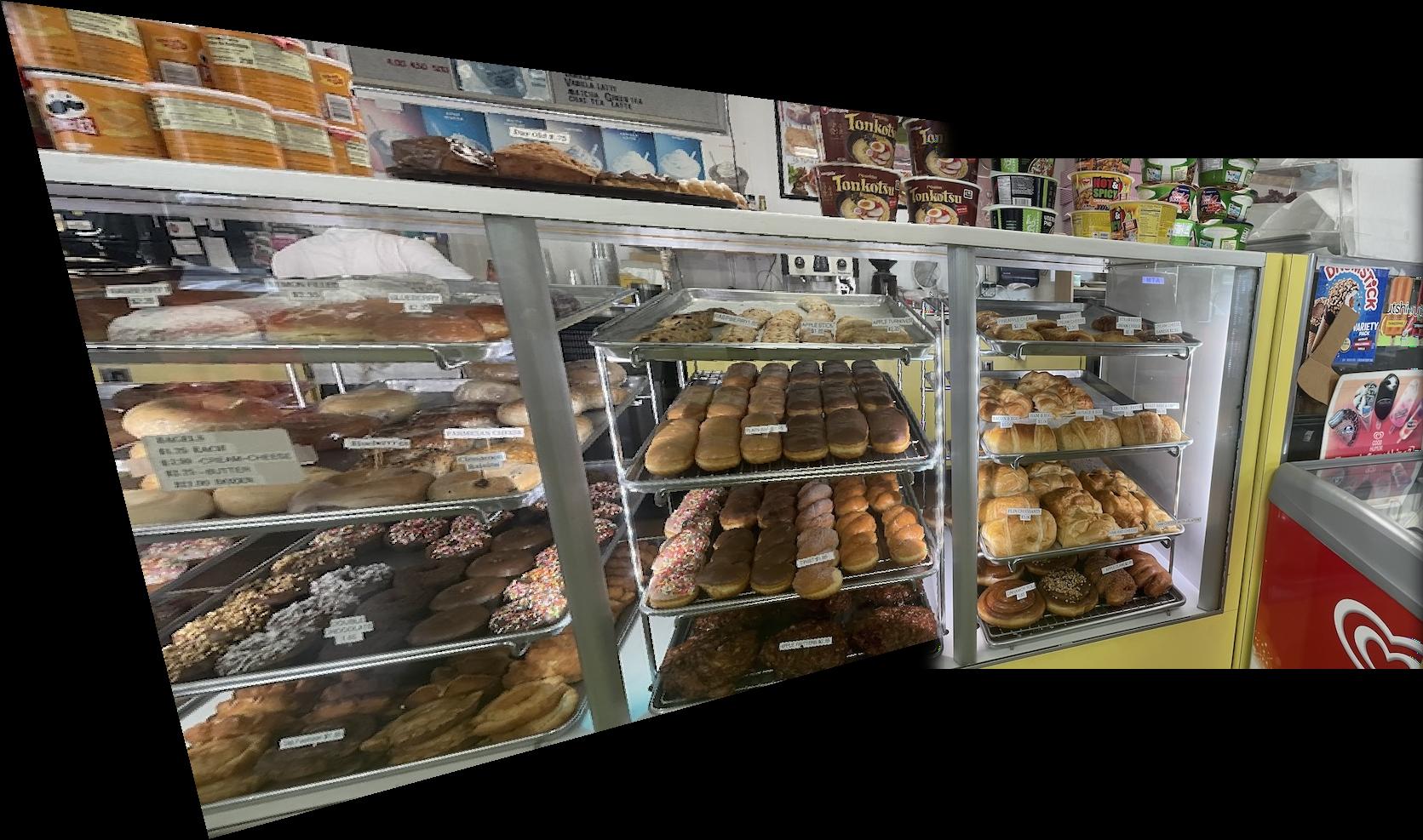
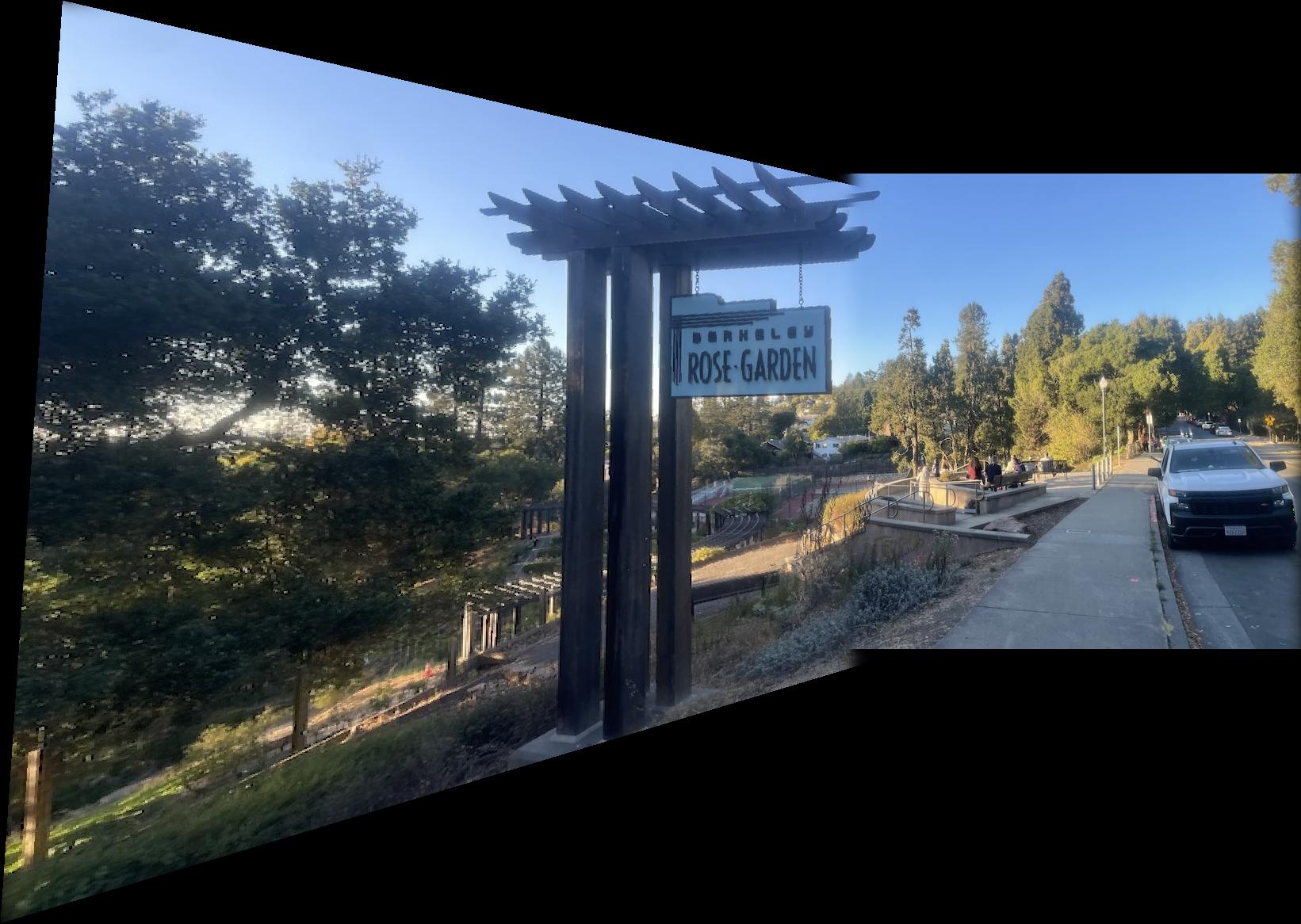
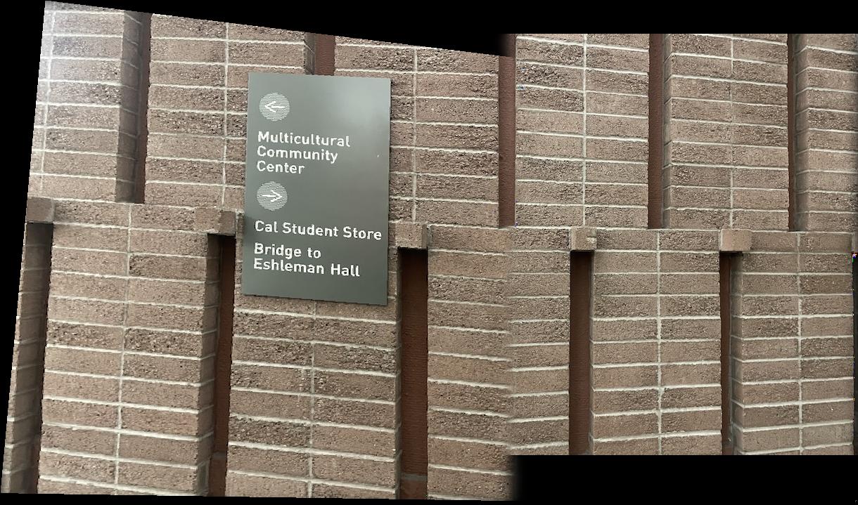
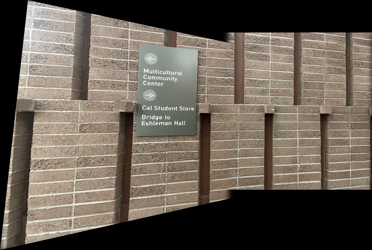
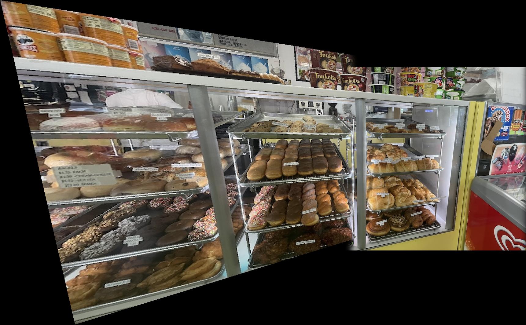
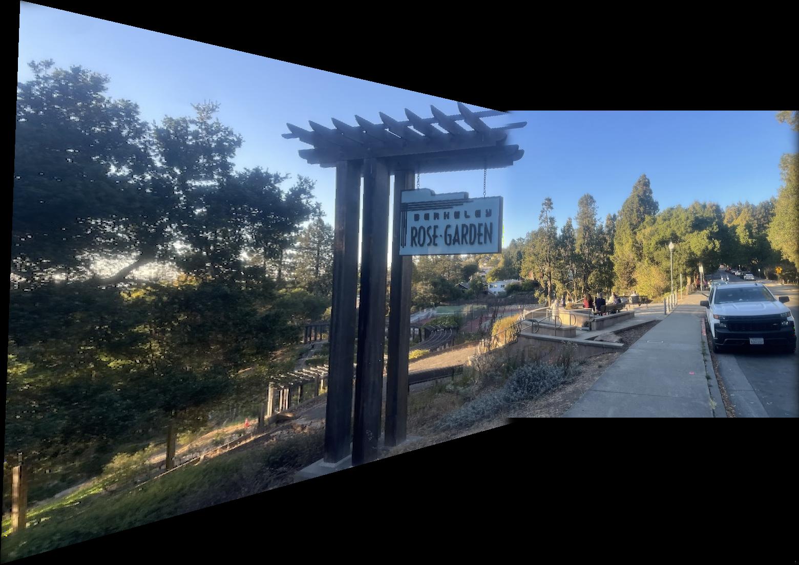
For creating the mosaics it’s the same as warping but we can use the point correspondences to refine our alignments and make our lives easier. Of course without any sort of blending this creates unpleasant artifacts:

For blending I reused my code from project 2, with laplacian/gaussian stacks of size 2 and sigma_start = 5. I tried a lot of things for the initial mask but usually what works best is just a line that divides the area where im1 and im2 intersect in 2.

More mosaics

Part B: Feature Matching for Autostitching

In this part, we implement automatic stitching following "Multi-Image Matching using Multi-Scale Oriented Patches" by Brown et al with simplifications.

Steps Involved

1. Detecting corner features in an image.
2. Extracting a Feature Descriptor for each feature point.
3. Matching these feature descriptors between two images.
4. Using a robust method (RANSAC) to compute a homography.

Image Resizing

I resized all my images to be about 600 x 800 pixels for efficiency and so that my “magic numbers” generalize better.

Detecting corner features in an image

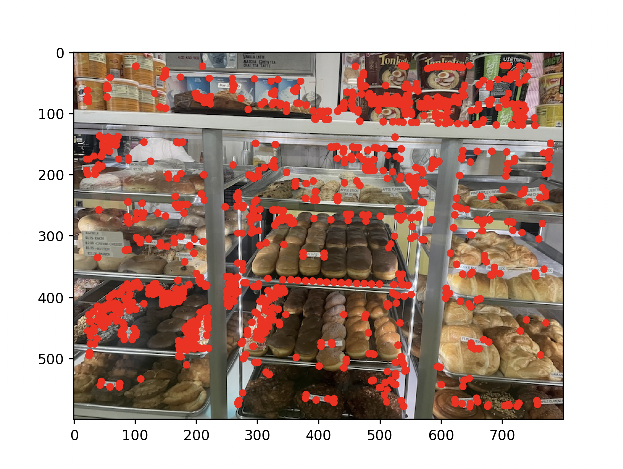
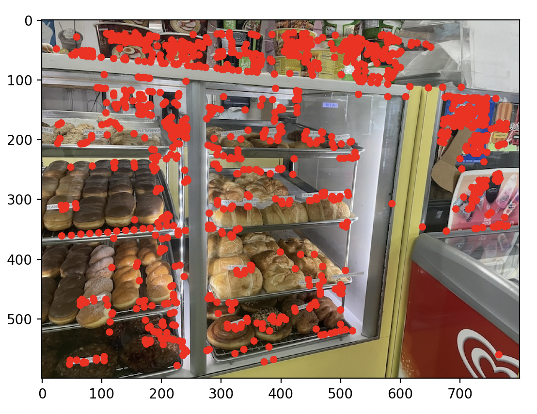
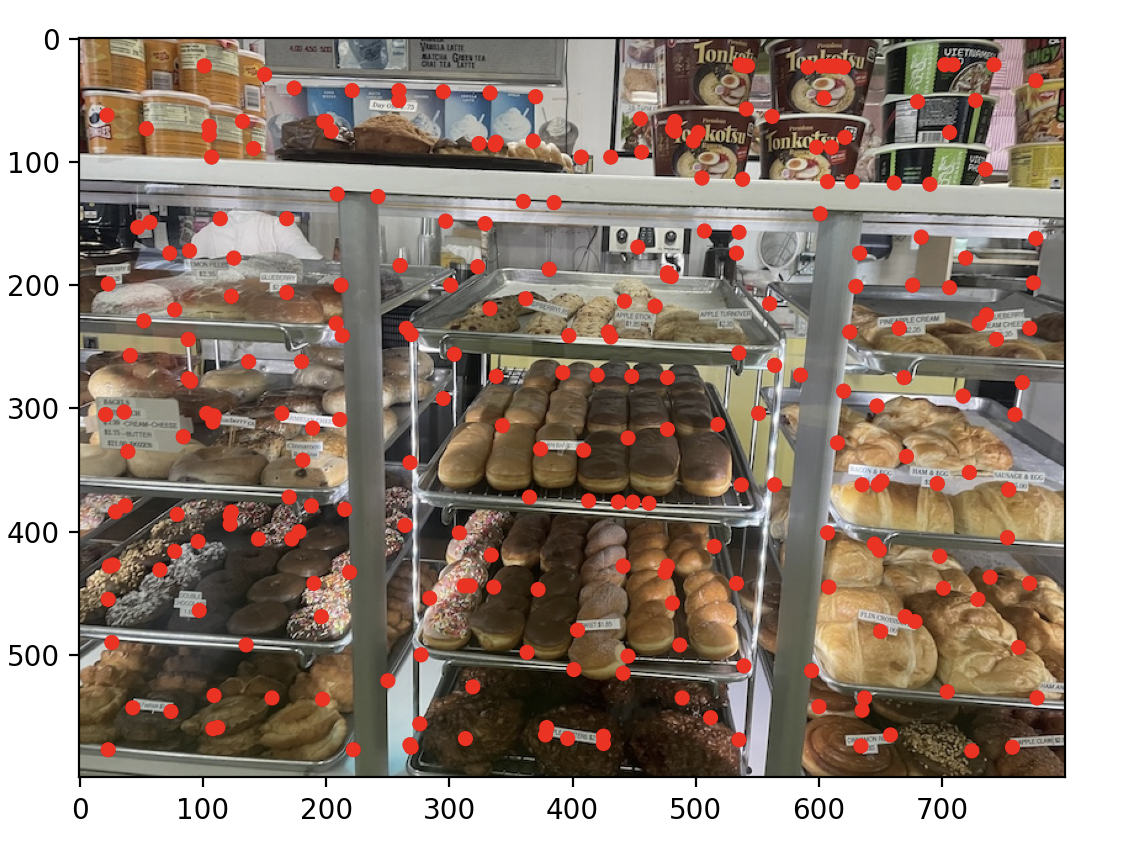
to detect corners in an image, I first used the provided in harris.py with a discarded edge of 20 pixels. Because the default settings took very long to run on large high-resolution images and produced an exorbitant number of points, I also set the min_dist parameter of peak_local_max to 5 so that fewer points are sampled. This still produced almost 120k points for my full resolution images, so I then chose the top 10k points based on their Harris response.

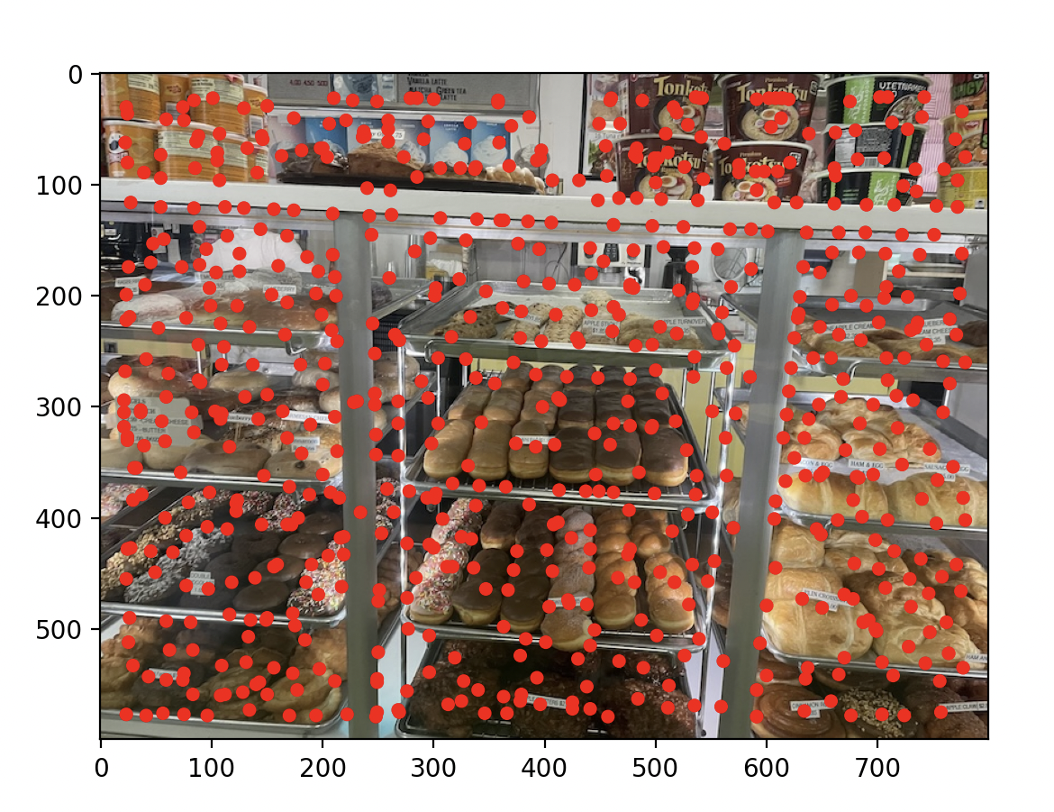
Just using Harris resulted in bad keypoints if n was small (too many clustered points) or just too many key points to be efficient. To solve this I did as the assignment recommended/demanded and implemented ANMS using kv trees. Conceptually the algorithm assigns every point a minimum radius at which that point is suppressed, this value is the local area where the point is strong. Then we filter by r.

r = 15 on the left, r = 25 on the right

Extracting a Feature Descriptor for each feature point

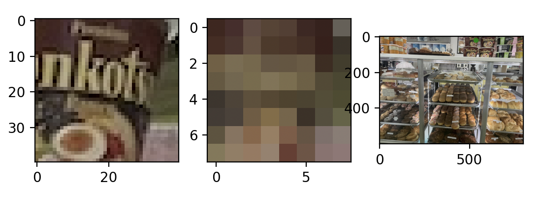
To match points across images the paper advises that we need more than just one pixel. Instead we construct feature descriptors of locations around our pixels (size 40 by 40) that we then down sample with anti aliasing grayscale patch (I also tried color). We then normalize the patch.

Here is an example, colorized for your viewing experience, the corresponding point in the image has been colored green

Matching these feature descriptors between two images

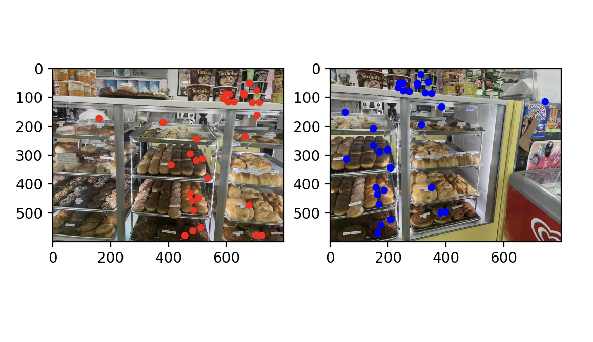
Once we have our feature descriptors we can run a nearest neighbor algorithm to find potential matches. Then, following the paper we can filter the matches by thresholding the value of nn(1)/nn(2) (closest match over second closest match). The Idea is that good points will have a good first match and will be easily distinguishable from their second match. I went with 0.5

Use a robust method (RANSAC) to compute a homography

Finally, we can use RANSAC to compute a homography with the following steps:

1. Select 4 random point pairs.
2. Compute a homography using these points.
3. Count the number of outliers where the distance is greater than some threshold epsilon.
4. Repeat steps 1-3 n times.
5. Return the best homography with the minimum number of outliers.

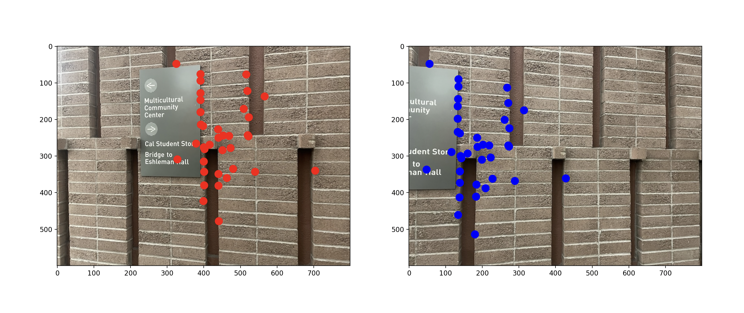
Here is an image of the inliers of my best homography (37 inliers)

Original on the left, Automatic on the right

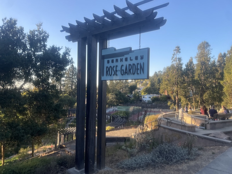
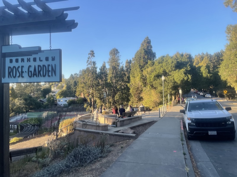
After carefully looking at the mosaics, I think the automatically generated ones are better in general (by a small amount). This is most evident in the “rose garden sign” mosaic when you look at the handrail.

Coolest thing I learned

Getting better at using kv trees was really cool, but I think the coolest thing I learned was how to rectify images, the example given in class about the painting blew my mind!

Original Pictures

Information

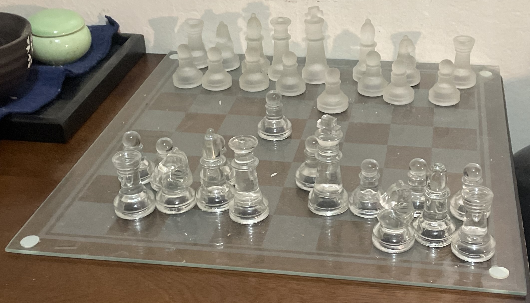
This website contains transitions not captured by the pdf, spesificaly, the title image changes into a high gamma verison and then into the black and white threshold filter version.